Histogram of Oriented Gradients, or HOG for short, are descriptors mainly used in computer vision and machine learning for object detection. However, we can also use HOG descriptors for quantifying and representing both shape and texture.
HOG features were first introduced by Dalal and Triggs in their CVPR 2005 paper, Histogram of Oriented Gradients for Human Detection. In their work, Dalal and Triggs proposed HOG and a 5-stage descriptor to classify humans in still images.
The 5 stages include:
- Normalizing the image prior to description.
- Computing gradients in both the x and y directions.
- Obtaining weighted votes in spatial and orientation cells.
- Contrast normalizing overlapping spatial cells.
- Collecting all Histograms of Oriented gradients to form the final feature vector.
The most important parameters for the HOG descriptor are the orientations , pixels_per_cell , and the cells_per_block . These three parameters (along with the size of the input image) effectively control the dimensionality of the resulting feature vector. We’ll be reviewing these parameters and their implications later in this article.
In most real-world applications, HOG is used in conjunction with a Linear SVM to perform object detection. The reason HOG is utilized so heavily is because local object appearance and shape can be characterized using the distribution of local intensity gradients. In fact, these are the exact same image gradients that we learned about in the Gradients lesson, but only now we are going to take these image gradients and turn them into a robust and powerful image descriptor.
We’ll be discussing the steps necessary to combine both HOG and a Linear SVM into an object classifier later in this course. But for now just understand that HOG is mainly used as a descriptor for object detection and that later these descriptors can be fed into a machine learning classifier.
HOG is implemented in both OpenCV and scikit-image. The OpenCV implementation is less flexible than the scikit-image implementation, and thus we will primarily used the scikit-image implementation throughout the rest of this course.
Objectives:
In this lesson, we will be discussing the Histogram of Oriented Gradients image descriptor in detail.
What are HOG descriptors used to describe?
HOG descriptors are mainly used to describe the structural shape and appearance of an object in an image, making them excellent descriptors for object classification. However, since HOG captures local intensity gradients and edge directions, it also makes for a good texture descriptor.
The HOG descriptor returns a real-valued feature vector. The dimensionality of this feature vector is dependent on the parameters chosen for the orientations , pixels_per_cell , and cells_per_block parameters mentioned above.
How do HOG descriptors work?
The cornerstone of the HOG descriptor algorithm is that appearance of an object can be modeled by the distribution of intensity gradients inside rectangular regions of an image:
Implementing this descriptor requires dividing the image into small connected regions called cells, and then for each cell, computing a histogram of oriented gradients for the pixels within each cell. We can then accumulate these histograms across multiple cells to form our feature vector.
Dalal and Triggs also demonstrated that we can perform block normalization to improve performance. To perform block normalization we take groups of overlapping cells, concatenate their histograms, calculate a normalizing value, and then contrast normalize the histogram. By normalizing over multiple, overlapping blocks, the resulting descriptor is more robust to changes in illumination and shadowing. Furthermore, performing this type of normalization implies that each of the cells will be represented in the final feature vector multiple times but normalized by a slightly different set of neighboring cells.
Now, let’s review each of the steps for computing the HOG descriptor.
Step 1: Normalizing the image prior to description.
This normalization step is entirely optional, but in some cases this step can improve performance of the HOG descriptor. There are three main normalization methods that we can consider:
- Gamma/power law normalization: In this case, we take the
of each pixel
in the input image. However, as Dalal and Triggs demonstrated, this approach is perhaps an “over-correction” and hurts performance.
- Square-root normalization: Here, we take the
of each pixel
- Variance normalization: A slightly less used form of normalization is variance normalization. Here, we compute both the mean
and standard deviation
of the input image. All pixels are mean centered by subtracting the mean from the pixel intensity, and then normalized through dividing by the standard deviation:
. Dalal and Triggs do not report accuracy on variance normalization; however, it is a form of normalization that I like to perform and thought it was worth including.
In most cases, it’s best to start with either no normalization or square-root normalization. Variance normalization is also worth consideration, but in most cases it will perform in a similar manner to square-root normalization (at least in my experience).
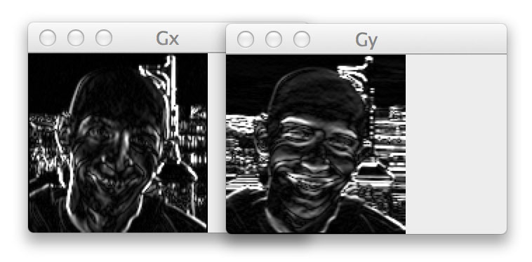
Step 2: Gradient computation
The first actual step in the HOG descriptor is to compute the image gradient in both the x and y direction. These calculations should seem familiar, as we have already reviewed them in the Gradients lesson.
We’ll apply a convolution operation to obtain the gradient images:
 and
and 
where 


As a matter of completeness, here is an example of computing both the x and y gradient of an input image:
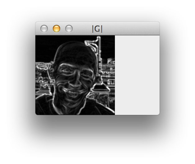
Now that we have our gradient images, we can compute the final gradient magnitude representation of the image:

Finally, the orientation of the gradient for each pixel in the input image can then be computed by:
")
Given both 

Step 3: Weighted votes in each cell
Now that we have our gradient magnitude and orientation representations, we need to divide our image up into cells and blocks.
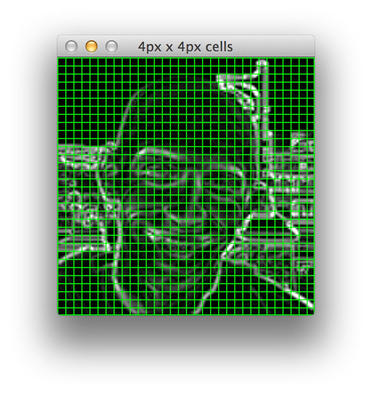
A “cell” is a rectangular region defined by the number of pixels that belong in each cell. For example, if we had a 128 x 128 image and defined our pixels_per_cell as 4 x 4, we would thus have 32 x 32 = 1024 cells:
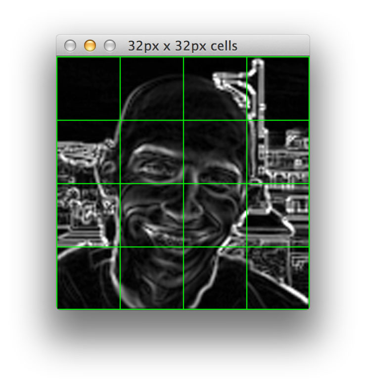
If we defined our pixels_per_cell as 32 x 32, we would have 4 x 4 = 16 total cells:
And if we defined pixels_per_cell to be 128 x 128, we would only have 1 total cell:
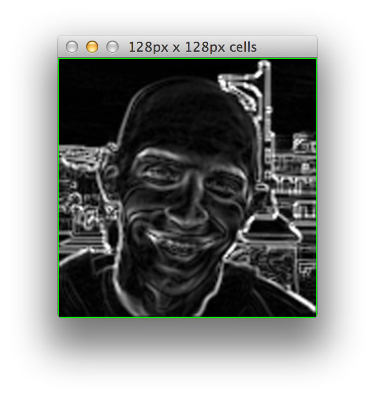
Obviously, this is quite an exaggerated example; we would likely never be interested in a 1 x 1 cell representation. Instead, this demonstrates how we can divide an image into cells based on the number of pixels per cell.
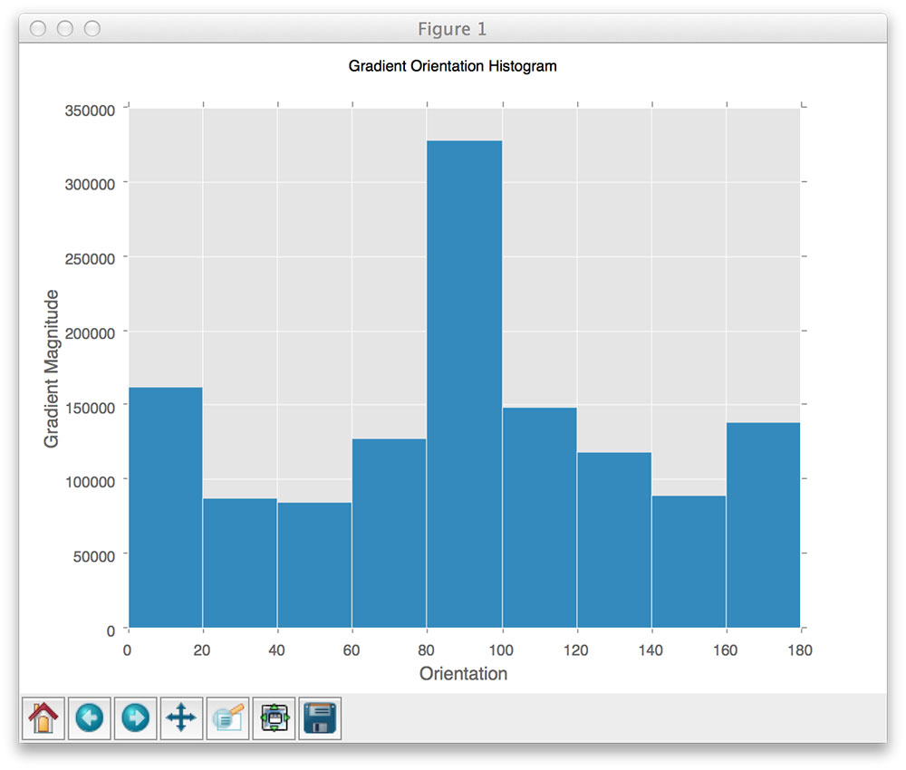
Now, for each of the cells in the image, we need to construct a histogram of oriented gradients using our gradient magnitude
But before we construct this histogram, we need to define our number of orientations . The number of orientations control the number of bins in the resulting histogram. The gradient angle is either within the range ![[0, 180]](https://s0.wp.com/latex.php?latex=%5B0%2C+180%5D&bg=ffffff&fg=000000&s=0 "[0, 180]")
![[0, 360]](https://s0.wp.com/latex.php?latex=%5B0%2C+360%5D&bg=ffffff&fg=000000&s=0 "[0, 360]")
![[9, 12]](https://s0.wp.com/latex.php?latex=%5B9%2C+12%5D&bg=ffffff&fg=000000&s=0 "[9, 12]")
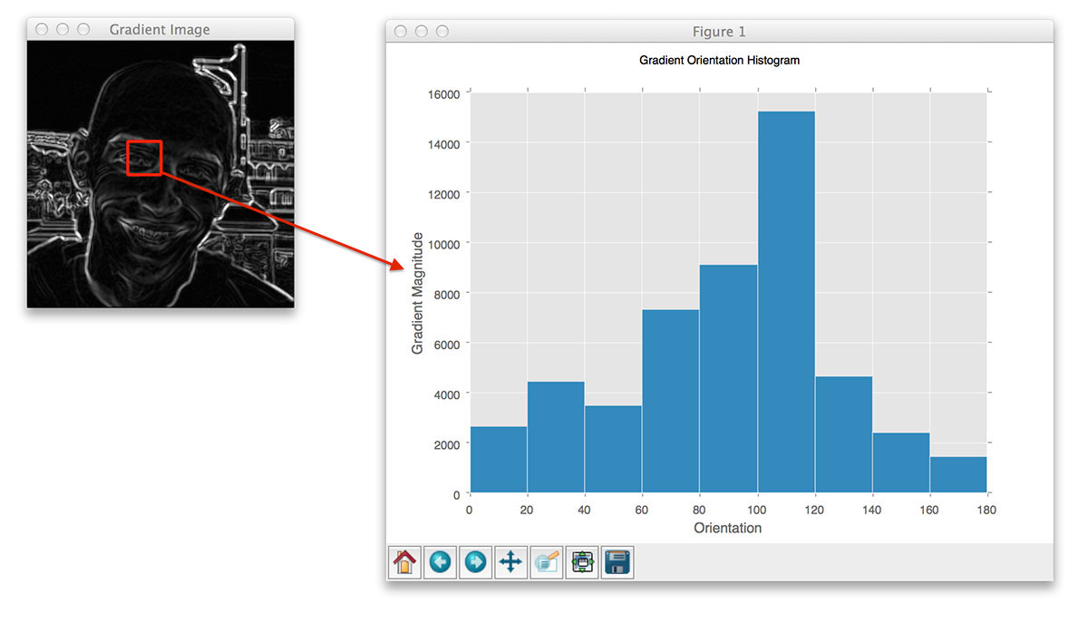
Finally, each pixel contributes a weighted vote to the histogram — the weight of the vote is simply the gradient magnitude
Let’s make this more clear by taking a look at our example image divided up into 16 x 16 pixel cells:

And then for each of these cells, we are going to compute a histogram of oriented gradients using 9 orientations (or bins) per histogram:
Here is a more revealing animation were we can visually see a different histogram computed for each of the cells:
At this point, we could collect and concatenated each of these histograms to form our final feature vector. However, it’s beneficial to apply block normalization, which we’ll review in the next section.
Step 4: Contrast normalization over blocks
To account for changes in illumination and contrast, we can normalize the gradient values locally. This requires grouping the “cells” together into larger, connecting “blocks”. It is common for these blocks to overlap, meaning that each cell contributes to the final feature vector more than once.
Again, the number of blocks are rectangular; however, our units are no longer pixels — they are the cells! Dalal and Triggs report that using either 2 x 2 or 3 x 3 cells_per_block obtains reasonable accuracy in most cases.
Here is an example where we have taken an input region of an image, computed a gradient histogram for each cell, and then locally grouped the cells into overlapping blocks:
For each of the cells in the current block we concatenate their corresponding gradient histograms, followed by either L1 or L2 normalizing the entire concatenated feature vector. Again, performing this type of normalization implies that each of the cells will be represented in the final feature vector multiple times but normalized by a different value. While this multi-representation is redundant and wasteful of space, it actually increases performance of the descriptor.
Finally, after all blocks are normalized, we take the resulting histograms, concatenate them, and treat them as our final feature vector.
Where are HOG descriptors implemented?
HOG descriptors are implemented inside the OpenCV and scikit-image library. However, the OpenCV implementation is not very flexible and is primarily geared towards the Dalal and Triggs implementation. The scikit-image implementation is far more flexible, and thus we will primarily use the scikit-image implementation throughout this course.
How do I use HOG descriptors?
Here is an example of how to compute HOG descriptors using scikit-image:
from skimage import feature
H = feature.hog(logo, orientations=9, pixels_per_cell=(8, 8),
	cells_per_block=(2, 2), transform_sqrt=True, block_norm="L1")
We can also visualize the resulting HOG image:
from skimage import exposure
from skimage import feature
import cv2

(H, hogImage) = feature.hog(logo, orientations=9, pixels_per_cell=(8, 8),
	cells_per_block=(2, 2), transform_sqrt=True, block_norm="L1",
	visualize=True)
hogImage = exposure.rescale_intensity(hogImage, out_range=(0, 255))
hogImage = hogImage.astype("uint8")

cv2.imshow("HOG Image", hogImage)
(2017-11-28) Update for skimage: In scikit-image==0.12 , the normalise parameter has been updated to transform_sqrt . The transform_sqrt performs the exact same operation, only with a different name. If you’re using an older version of scikit-image (again, before the v0.12 release), then you’ll want to change transform_sqrt to normalise . In scikit-image==0.15 the default value of block_norm=”L1″ has been deprecated and changed to block_norm=”L2-Hys” . Therefore, for this lesson we’ll explicitly specify block_norm=”L1″ . Doing this will avoid it switching to “L2-Hys” with version updates without us knowing (and yielding incorrect car logo identification results). You can read about L1 and L2 norms here.
(2019-01-06) Update for skimage: The visualise parameter is deprecated and changed to visualize .
Identifying car logos using HOG descriptors
Later on in the PyImageSearch Gurus course, we’ll learn how to automatically detect and recognize license plates in images.
But what if we could also identify the brand of car based on its logo?
Now that would be pretty cool.
In the remainder of this lesson, I’ll demonstrate how we can use the Histogram of Oriented Gradients descriptor to characterize the logos of car brands. Just like in the Haralick texture lesson, we’ll be leveraging a bit of machine learning to aide us in the classification (which is a pretty common practice when it comes to identifying non-trivial shapes and objects).
Again, I won’t be performing a deep dive on the (very small amount of) machine learning we’ll be using in this lesson — we have the entire Image Classification module for that. If by the end of this lesson there are a couple of lines of code that feel a little bit like “black box magic” to you, that’s okay and to be expected. Remember, the point of these image descriptor lessons is providing a quick demonstration of how you can use them in your own applications. The rest of the modules in the PyImageSearch Gurus course will help fill in any gaps.
But before we dive deep into this project, let’s look at our dataset.
Dataset
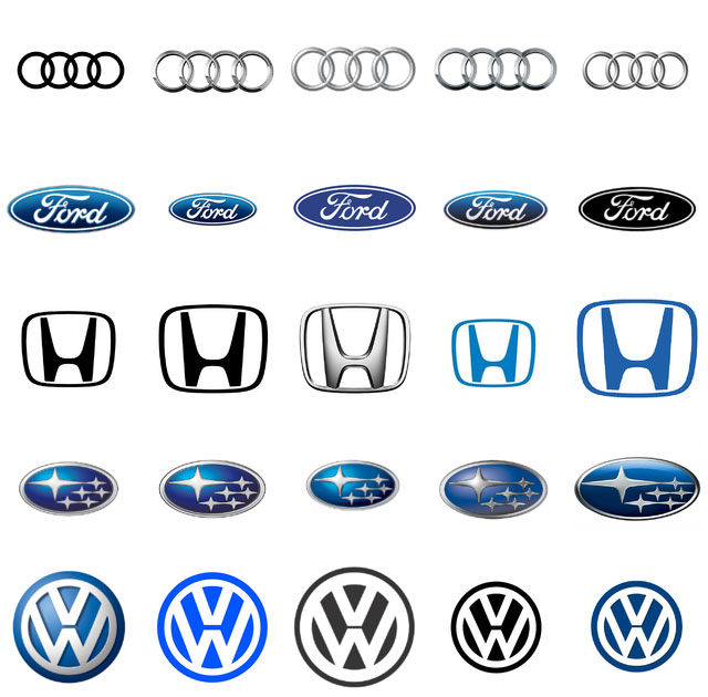
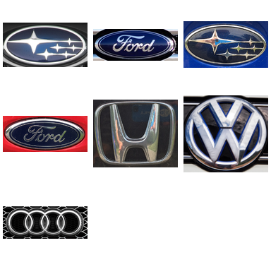
Our car logo dataset consists of five brands of vehicles: Audi, Ford, Honda, Subaru, and Volkswagen.
For each of these brands, I gathered five training images from Google. These images are the example images we’ll use to teach our machine learning algorithm what each of the car logos look like. Our training dataset can be seen below:
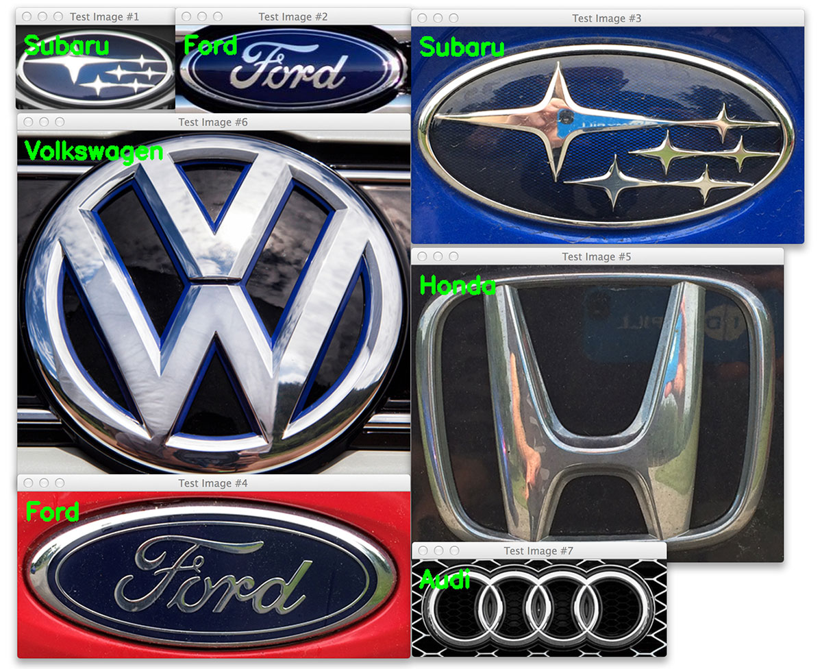
After gathering the images from Google, I then went outside and took a stroll around the local parking lot, snapping seven photos of car logos. These logos will serve as our test set that we can use to evaluate the performance of our classifier. The seven testing images are displayed below:
Our goal
The goal of this project is to:
- Extract HOG features from our training set to characterize and quantify each car logo.
- Train a machine learning classifier to distinguish between each car logo.
- Apply a classifier to recognize new, unseen car logos.
Recognizing car logos
Alright, enough talk. Let’s start coding up this example. Open up a new file, name it recognize_car_logos.py , and let’s get coding:
# import the necessary packages
from sklearn.neighbors import KNeighborsClassifier
from skimage import exposure
from skimage import feature
from imutils import paths
import argparse
import imutils
import cv2

# construct the argument parse and parse command line arguments
ap = argparse.ArgumentParser()
ap.add_argument("-d", "--training", required=True, help="Path to the logos training dataset")
ap.add_argument("-t", "--test", required=True, help="Path to the test dataset")
args = vars(ap.parse_args())

# initialize the data matrix and labels
print("[INFO] extracting features...")
data = []
labels = []
This code should look fairly similar to our code from the Haralick texture example. Parsing our command line arguments, we can see that we need two switches. The first is –training , which is the path to where the example car logos reside on disk. The second switch is –test , the path to our directory of testing images we’ll use to evaluate our car logo classifier.
We’ll also initialize data and labels , two lists that will hold the HOG features and car brand name for each image in our training set, respectively.
Let’s go ahead and extract HOG features from our training set:
# loop over the image paths in the training set
for imagePath in paths.list_images(args["training"]):
	# extract the make of the car
	make = imagePath.split("/")[-2]

	# load the image, convert it to grayscale, and detect edges
	image = cv2.imread(imagePath)
	gray = cv2.cvtColor(image, cv2.COLOR_BGR2GRAY)
	edged = imutils.auto_canny(gray)

	# find contours in the edge map, keeping only the largest one which
	# is presmumed to be the car logo
	cnts = cv2.findContours(edged.copy(), cv2.RETR_EXTERNAL,
		cv2.CHAIN_APPROX_SIMPLE)
	cnts = imutils.grab_contours(cnts)
	c = max(cnts, key=cv2.contourArea)

	# extract the logo of the car and resize it to a canonical width
	# and height
	(x, y, w, h) = cv2.boundingRect(c)
	logo = gray[y:y + h, x:x + w]
	logo = cv2.resize(logo, (200, 100))

	# extract Histogram of Oriented Gradients from the logo
	H = feature.hog(logo, orientations=9, pixels_per_cell=(10, 10),
		cells_per_block=(2, 2), transform_sqrt=True, block_norm="L1")

	# update the data and labels
	data.append(H)
	labels.append(make)
On Line 22, we start looping over each of the image paths in the training directory. An example image path looks like this: car_logos/audi/audi_01.png
Using this image path, we are able to extract the make of the car on Line 24 by splitting the path and extracting the second sub-directory name, or in this case audi .
From there, we’ll perform a bit of pre-processing and prepare the car logo to be described using the Histogram of Oriented Gradients descriptor. All we need to do is load the image from disk, convert it to grayscale, and then use our handy auto_canny function to detect edges in the brand logo:
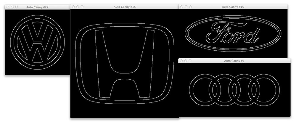
Notice how in each case we are able to find the outline of the car logo.
Anytime we detect an outline, you can be sure that the next step is (almost always) to find the contour of the outline. In fact, that is exactly what Lines 33-36 do — extract the largest contour in the edge map, assumed to be the outline of the car logo.
Lines 40 and 41 then take the largest contour region, compute the bounding box, and extract the ROI.
Be sure to pay attention to Line 42, because it’s extremely important. As I mentioned earlier in this lesson, having various widths and heights for your image can lead to HOG feature vectors of different sizes — in nearly all situations this is not the intended behavior that you want!
Think of it this way: let’s assume that I extracted a HOG feature vector of size 1,024-d from Image A. And then I extracted a HOG feature vector (using the exact same HOG parameters) from Image B, which had different dimensions (i.e. width and height) than Image A, leaving me with a feature vector of size 512-d.
How would I go about comparing these two feature vectors?
The short answer is that you can’t.
Remember, our extracted feature vectors are supposed to characterize and represent the visual contents of an image. And if our feature vectors are not the same dimensionality, then they cannot be compared for similarity. And if we cannot compare our feature vectors for similarity, we are unable to compare our two images at all!
Because of this, when extracting HOG features from a dataset of images, you’ll want to define a canonical, known size that each image will be resized to. In many cases, this means that you’ll be throwing away the aspect ratio of the image. Normally, destroying the aspect ratio of an image should be avoided — but in this case we are happy to do it, because it ensures (1) that each image in our dataset is described in a consistent manner, and (2) each feature vector is of the same dimensionality. We’ll be discussing this point much more when we reach the Custom Object Detector module.
Anyway, now that our logo is resized to a known, pre-defined 200 x 100 pixels, we can then apply the HOG descriptor using orientations=9 , pixels_per_cell=(10, 10) , cells_per_block=(2, 2) , and square-root normalization. These parameters were obtained by experimentation and examining the accuracy of the classifier — you should expect to do this as well whenever you use the HOG descriptor. Running experiments and tuning the HOG parameters based on these parameters is a critical component in obtaining an accurate classifier.
Finally, given the HOG feature vector, we then update our data matrix and labels list with the feature vector and car make, respectively.
Given our data and labels we can now train our classifier:
# "train" the nearest neighbors classifier
print("[INFO] training classifier...")
model = KNeighborsClassifier(n_neighbors=1)
model.fit(data, labels)
print("[INFO] evaluating...")
To recognize and distinguish the difference between our five car brands, we are going to use scikit-learns KNeighborsClassifier.
The k-nearest neighbor classifier is a type of “lazy learning” algorithm where nothing is actually “learned”. Instead, the k-Nearest Neighbor (k-NN) training phase simply accepts a set of feature vectors and labels and stores them — that’s it! Then, when it is time to classify a new feature vector, it accepts the feature vector, computes the distance to all stored feature vectors (normally using the Euclidean distance, but any distance metric or similarity metric can be used), sorts them by distance, and returns the top k “neighbors” to the input feature vector. From there, each of the k neighbors vote as to what they think the label of the classification is. You can read more about the k-NN algorithm in this lesson.
In our case, we are simply passing the HOG feature vectors and labels to our k-NN algorithm and ask it to report back what is the closest logo to our query features using k=1 neighbors.
Let’s see how we can use our k-NN classifier to recognize various car logos:
# loop over the test dataset
for (i, imagePath) in enumerate(paths.list_images(args["test"])):
	# load the test image, convert it to grayscale, and resize it to
	# the canonical size
	image = cv2.imread(imagePath)
	gray = cv2.cvtColor(image, cv2.COLOR_BGR2GRAY)
	logo = cv2.resize(gray, (200, 100))

	# extract Histogram of Oriented Gradients from the test image and
	# predict the make of the car
	(H, hogImage) = feature.hog(logo, orientations=9, pixels_per_cell=(10, 10),
		cells_per_block=(2, 2), transform_sqrt=True, block_norm="L1", visualize=True)
	pred = model.predict(H.reshape(1, -1))[0]

	# visualize the HOG image
	hogImage = exposure.rescale_intensity(hogImage, out_range=(0, 255))
	hogImage = hogImage.astype("uint8")
	cv2.imshow("HOG Image #{}".format(i + 1), hogImage)

	# draw the prediction on the test image and display it
	cv2.putText(image, pred.title(), (10, 35), cv2.FONT_HERSHEY_SIMPLEX, 1.0,
		(0, 255, 0), 3)
	cv2.imshow("Test Image #{}".format(i + 1), image)
	cv2.waitKey(0)
Line 59 starts looping over the images in our testing set. For each of these images, we’ll load it from disk; convert it to grayscale; resize it to a known, fixed size; and then extract HOG feature vectors from it in the exact same manner as we did in the training phase (Lines 62-69).
Line 70 then makes a call to our k-NN classifier, passing in our HOG feature vector for the current testing image and asking the classifier what it thinks the logo is.
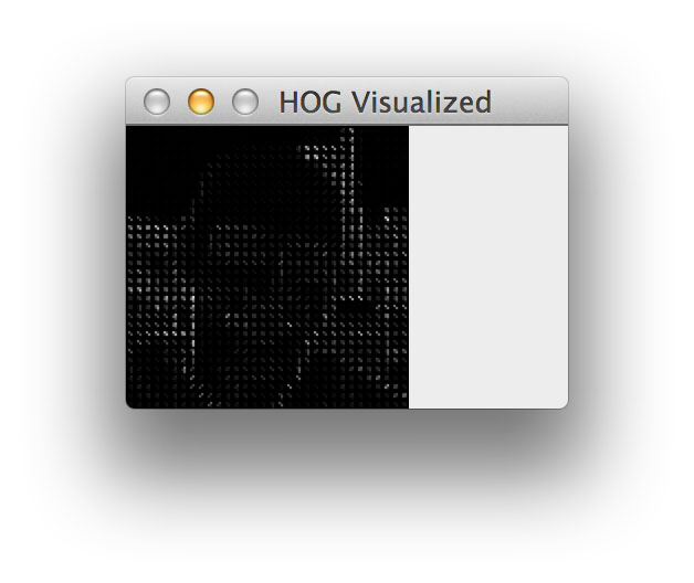
We can also visualize our Histogram of Oriented Gradients image on Lines 73-75. This is especially useful when debugging your HOG parameters to ensure the contents of our image are being adequately quantified. Below are some examples of the HOG image our testing car logos:
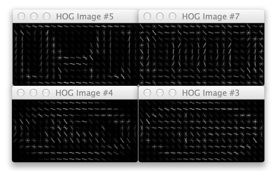
Notice how the HOG image is always 200 x 100 pixels, which are the dimensions of our resized testing image. We can also see how the pixels_per_cell and orientations parameters come into play here, as well as the dominant orientation of each cell, where the size of the cell is defined by the pixels_per_cell . The more pixels in the pixels_per_cell , the more coarse our representation is. And similarly, smaller values of pixels_per_cell will yield more fine-grained representations. Visualizing a HOG image is an excellent way to “see” what your HOG descriptor and parameter set is describing.
Finally, we take the result of the classification, draw it on our test image, and display it to our screen on Lines 78-81.
To give our car logo classifier a try, simply open up your terminal and execute the following command:
$ python recognize_car_logos.py --training car_logos --test test_images
And below you’ll see our output classification:
In each case, we were able to correctly classify the brand of car using HOG features!
Of course, this approach only worked, because we had a tight cropping of the car logo. If we had described the entire image of a car, it is very unlikely that we would have been able to correctly classify the brand. But again, that’s something we can resolve when we get to the Custom Object Detector module, specifically sliding windows and image pyramids.
In the meantime, this example was still able to demonstrate how to use the Histogram of Oriented Gradients descriptor and the k-NN classifier to recognize the logos of cars. The key takeaway here is that if you can consistently detect and extract the ROI of your image dataset, the HOG descriptor should definitely be on your list of image descriptors to apply, as it’s very powerful and able to obtain good results, especially when applied in conjunction with machine learning.
Suggestions when using HOG descriptors:
HOG descriptors are very powerful; however, it can be tedious to choose the correct parameters for the number of orientations , pixels_per_cell , and cells_per_block , especially when you start working with object classification.
As a starting point, I tend to use orientations=9 , pixels_per_cell=(4, 4) , and cells_per_block=(2, 2) , then go from there. It’s unlikely that your first set of parameters will yield the best performance; however, it’s important to start somewhere and obtain a baseline — results can be improved via parameter tuning.
It’s also important to resize your image to a reasonable size. If your input region is 32 x 32 pixels, then the resulting dimensionality would be 1,764-d. But if your input region is 128 x 128 pixel and you again used the above parameters, your feature vector would be 34,596-d! By using large image regions and not paying attention to your HOG parameters, you can end up with extremely large feature vectors.
We’ll be utilizing HOG descriptors later in this course for object classification, so if you’re a little confused on how to properly tune the parameters, don’t worry — this won’t be the last time you see these descriptors!
HOG Pros and Cons
Pros:
- Very powerful descriptor.
- Excellent at representing local appearance.
- Extremely useful for representing structural objects that do not demonstrate substantial variation in form (i.e. buildings, people walking the street, bicycles leaning against a wall).
- Very accurate for object classification.
Cons:
- Can result in very large feature vectors, leading to large storage costs and computationally expensive feature vector comparisons.
- Often non-trivial to tune the orientations , pixels_per_cell , and cells_per_block parameters.
- Not the slowest descriptor to compute, but also nowhere near the fastest.
- If the object to be described exhibits substantial structural variation (i.e. the rotation/orientation of the object is consistently different), then the standard vanilla implementation of HOG will not perform well.