Combining Data From Multiple Excel Files
Posted by Chris Moffitt in articles
Introduction
A common task for python and pandas is to automate the process of aggregating data from multiple files and spreadsheets.
This article will walk through the basic flow required to parse multiple Excel files, combine the data, clean it up and analyze it. The combination of python + pandas can be extremely powerful for these activities and can be a very useful alternative to the manual processes or painful VBA scripts frequently used in business settings today.
The Problem
Before, I get into the examples, here is a simple diagram showing the challenges with the common process used in businesses all over the world to consolidate data from multiple Excel files, clean it up and perform some analysis.
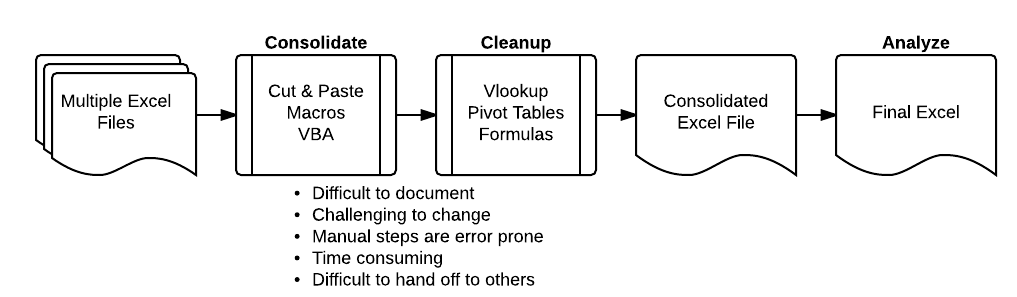
If you’re reading this article, I suspect you have experienced some of the problems shown above. Cutting and pasting data or writing painful VBA code will quickly get old. There has to be a better way!
Python + pandas can be a great alternative that is much more scaleable and powerful.
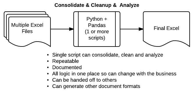
By using a python script, you can develop a more streamlined and repeatable solution to your data processing needs. The rest of this article will show a simple example of how this process works. I hope it will give you ideas of how to apply these tools to your unique situation.
Collecting the Data
If you are interested in following along, here are the excel files and a link to the notebook:
The first step in the process is collecting all the data into one place.
First, import pandas and numpy
import pandas as pd
import numpy as np
Let’s take a look at the files in our input directory, using the convenient shell commands in ipython.
!ls ../in
address-state-example.xlsx  report.xlsx                sample-address-new.xlsx
customer-status.xlsx            sales-feb-2014.xlsx    sample-address-old.xlsx
excel-comp-data.xlsx            sales-jan-2014.xlsx    sample-diff-1.xlsx
my-diff-1.xlsx                  sales-mar-2014.xlsx    sample-diff-2.xlsx
my-diff-2.xlsx                  sample-address-1.xlsx  sample-salesv3.xlsx
my-diff.xlsx                    sample-address-2.xlsx
pricing.xlsx                    sample-address-3.xlsx
There are a lot of files, but we only want to look at the sales .xlsx files.
!ls ../in/sales*.xlsx
../in/sales-feb-2014.xlsx ../in/sales-jan-2014.xlsx ../in/sales-mar-2014.xlsx
Use the python
glob
module to easily list out the files we need.
import glob
glob.glob("../in/sales*.xlsx")
['../in/sales-jan-2014.xlsx',
 '../in/sales-mar-2014.xlsx',
 '../in/sales-feb-2014.xlsx']
This gives us what we need. Let’s import each of our files and combine
them into one file.
Panda’s
concat
and
append
can do this for us. I’m going to use
append
in
this example.
The code snippet below will initialize a blank DataFrame then append all
of the individual files into the
all_data
DataFrame.
all_data = pd.DataFrame()
for f in glob.glob("../in/sales*.xlsx"):
    df = pd.read_excel(f)
    all_data = all_data.append(df,ignore_index=True)
Now we have all the data in our
all_data
DataFrame. You can use
describe
to look at it and make sure you data looks good.
all_data.describe()
| account number | quantity | unit price | ext price | |
|---|---|---|---|---|
| count | 1742.000000 | 1742.000000 | 1742.000000 | 1742.000000 |
| mean | 485766.487945 | 24.319173 | 54.985454 | 1349.229392 |
| std | 223750.660792 | 14.502759 | 26.108490 | 1094.639319 |
| min | 141962.000000 | -1.000000 | 10.030000 | -97.160000 |
| 25% | 257198.000000 | 12.000000 | 32.132500 | 468.592500 |
| 50% | 527099.000000 | 25.000000 | 55.465000 | 1049.700000 |
| 75% | 714466.000000 | 37.000000 | 77.607500 | 2074.972500 |
| max | 786968.000000 | 49.000000 | 99.850000 | 4824.540000 |
A lot of this data may not make much sense for this data set but I’m most interested in the count row to make sure the number of data elements makes sense. In this case, I see all the data rows I expect.
all_data.head()
| account number | name | sku | quantity | unit price | ext price | date | |
|---|---|---|---|---|---|---|---|
| 0 | 740150 | Barton LLC | B1-20000 | 39 | 86.69 | 3380.91 | 2014-01-01 07:21:51 |
| 1 | 714466 | Trantow-Barrows | S2-77896 | -1 | 63.16 | -63.16 | 2014-01-01 10:00:47 |
| 2 | 218895 | Kulas Inc | B1-69924 | 23 | 90.70 | 2086.10 | 2014-01-01 13:24:58 |
| 3 | 307599 | Kassulke, Ondricka and Metz | S1-65481 | 41 | 21.05 | 863.05 | 2014-01-01 15:05:22 |
| 4 | 412290 | Jerde-Hilpert | S2-34077 | 6 | 83.21 | 499.26 | 2014-01-01 23:26:55 |
It is not critical in this example but the best practice is to convert the date column to a date time object.
all_data['date'] = pd.to_datetime(all_data['date'])
Combining Data
Now that we have all of the data into one DataFrame, we can do any manipulations the DataFrame supports. In this case, the next thing we want to do is read in another file that contains the customer status by account. You can think of this as a company’s customer segmentation strategy or some other mechanism for identifying their customers.
First, we read in the data.
status = pd.read_excel("../in/customer-status.xlsx")
status
| account number | name | status | |
|---|---|---|---|
| 0 | 740150 | Barton LLC | gold |
| 1 | 714466 | Trantow-Barrows | silver |
| 2 | 218895 | Kulas Inc | bronze |
| 3 | 307599 | Kassulke, Ondricka and Metz | bronze |
| 4 | 412290 | Jerde-Hilpert | bronze |
| 5 | 729833 | Koepp Ltd | silver |
| 6 | 146832 | Kiehn-Spinka | silver |
| 7 | 688981 | Keeling LLC | silver |
| 8 | 786968 | Frami, Hills and Schmidt | silver |
| 9 | 239344 | Stokes LLC | gold |
| 10 | 672390 | Kuhn-Gusikowski | silver |
| 11 | 141962 | Herman LLC | gold |
| 12 | 424914 | White-Trantow | silver |
| 13 | 527099 | Sanford and Sons | bronze |
| 14 | 642753 | Pollich LLC | bronze |
| 15 | 257198 | Cronin, Oberbrunner and Spencer | gold |
We want to merge this data with our concatenated data set of sales. Use panda’s
merge
function and tell it to do a left join which is similar to Excel’s vlookup function.
all_data_st = pd.merge(all_data, status, how='left')
all_data_st.head()
| account number | name | sku | quantity | unit price | ext price | date | status | |
|---|---|---|---|---|---|---|---|---|
| 0 | 740150 | Barton LLC | B1-20000 | 39 | 86.69 | 3380.91 | 2014-01-01 07:21:51 | gold |
| 1 | 714466 | Trantow-Barrows | S2-77896 | -1 | 63.16 | -63.16 | 2014-01-01 10:00:47 | silver |
| 2 | 218895 | Kulas Inc | B1-69924 | 23 | 90.70 | 2086.10 | 2014-01-01 13:24:58 | bronze |
| 3 | 307599 | Kassulke, Ondricka and Metz | S1-65481 | 41 | 21.05 | 863.05 | 2014-01-01 15:05:22 | bronze |
| 4 | 412290 | Jerde-Hilpert | S2-34077 | 6 | 83.21 | 499.26 | 2014-01-01 23:26:55 | bronze |
This looks pretty good but let’s look at a specific account.
all_data_st[all_data_st["account number"]==737550].head()
| account number | name | sku | quantity | unit price | ext price | date | status | |
|---|---|---|---|---|---|---|---|---|
| 9 | 737550 | Fritsch, Russel and Anderson | S2-82423 | 14 | 81.92 | 1146.88 | 2014-01-03 19:07:37 | NaN |
| 14 | 737550 | Fritsch, Russel and Anderson | B1-53102 | 23 | 71.56 | 1645.88 | 2014-01-04 08:57:48 | NaN |
| 26 | 737550 | Fritsch, Russel and Anderson | B1-53636 | 42 | 42.06 | 1766.52 | 2014-01-08 00:02:11 | NaN |
| 32 | 737550 | Fritsch, Russel and Anderson | S1-27722 | 20 | 29.54 | 590.80 | 2014-01-09 13:20:40 | NaN |
| 42 | 737550 | Fritsch, Russel and Anderson | S1-93683 | 22 | 71.68 | 1576.96 | 2014-01-11 23:47:36 | NaN |
This account number was not in our status file, so we have a bunch of
NaN’s. We can decide how we want to handle this situation. For this
specific case, let’s label all missing accounts as bronze. Use the
fillna
function to easily accomplish this on the status column.
all_data_st['status'].fillna('bronze',inplace=True)
all_data_st.head()
| account number | name | sku | quantity | unit price | ext price | date | status | |
|---|---|---|---|---|---|---|---|---|
| 0 | 740150 | Barton LLC | B1-20000 | 39 | 86.69 | 3380.91 | 2014-01-01 07:21:51 | gold |
| 1 | 714466 | Trantow-Barrows | S2-77896 | -1 | 63.16 | -63.16 | 2014-01-01 10:00:47 | silver |
| 2 | 218895 | Kulas Inc | B1-69924 | 23 | 90.70 | 2086.10 | 2014-01-01 13:24:58 | bronze |
| 3 | 307599 | Kassulke, Ondricka and Metz | S1-65481 | 41 | 21.05 | 863.05 | 2014-01-01 15:05:22 | bronze |
| 4 | 412290 | Jerde-Hilpert | S2-34077 | 6 | 83.21 | 499.26 | 2014-01-01 23:26:55 | bronze |
Check the data just to make sure we’re all good.
all_data_st[all_data_st["account number"]==737550].head()
| account number | name | sku | quantity | unit price | ext price | date | status | |
|---|---|---|---|---|---|---|---|---|
| 9 | 737550 | Fritsch, Russel and Anderson | S2-82423 | 14 | 81.92 | 1146.88 | 2014-01-03 19:07:37 | bronze |
| 14 | 737550 | Fritsch, Russel and Anderson | B1-53102 | 23 | 71.56 | 1645.88 | 2014-01-04 08:57:48 | bronze |
| 26 | 737550 | Fritsch, Russel and Anderson | B1-53636 | 42 | 42.06 | 1766.52 | 2014-01-08 00:02:11 | bronze |
| 32 | 737550 | Fritsch, Russel and Anderson | S1-27722 | 20 | 29.54 | 590.80 | 2014-01-09 13:20:40 | bronze |
| 42 | 737550 | Fritsch, Russel and Anderson | S1-93683 | 22 | 71.68 | 1576.96 | 2014-01-11 23:47:36 | bronze |
Now we have all of the data along with the status column filled in. We can do our normal data manipulations using the full suite of pandas capability.
Using Categories
One of the relatively new functions in pandas is support for categorical data. From the pandas, documentation:
Categoricals are a pandas data type, which correspond to categorical variables in statistics: a variable, which can take on only a limited, and usually fixed, number of possible values (categories; levels in R). Examples are gender, social class, blood types, country affiliations, observation time or ratings via Likert scales.
For our purposes, the status field is a good candidate for a category type.
pd.__version__
'0.15.2'
First, we typecast it the column to a category using
astype
.
all_data_st["status"] = all_data_st["status"].astype("category")
This doesn’t immediately appear to change anything yet.
all_data_st.head()
| account number | name | sku | quantity | unit price | ext price | date | status | |
|---|---|---|---|---|---|---|---|---|
| 0 | 740150 | Barton LLC | B1-20000 | 39 | 86.69 | 3380.91 | 2014-01-01 07:21:51 | gold |
| 1 | 714466 | Trantow-Barrows | S2-77896 | -1 | 63.16 | -63.16 | 2014-01-01 10:00:47 | silver |
| 2 | 218895 | Kulas Inc | B1-69924 | 23 | 90.70 | 2086.10 | 2014-01-01 13:24:58 | bronze |
| 3 | 307599 | Kassulke, Ondricka and Metz | S1-65481 | 41 | 21.05 | 863.05 | 2014-01-01 15:05:22 | bronze |
| 4 | 412290 | Jerde-Hilpert | S2-34077 | 6 | 83.21 | 499.26 | 2014-01-01 23:26:55 | bronze |
Buy you can see that it is a new data type.
all_data_st.dtypes
account number             int64
name                      object
sku                       object
quantity                   int64
unit price               float64
ext price                float64
date              datetime64[ns]
status                  category
dtype: object
Categories get more interesting when you assign order to the categories.
Right now, if we call
sort
on the column, it will sort alphabetically.
all_data_st.sort(columns=["status"]).head()
| account number | name | sku | quantity | unit price | ext price | date | status | |
|---|---|---|---|---|---|---|---|---|
| 1741 | 642753 | Pollich LLC | B1-04202 | 8 | 95.86 | 766.88 | 2014-02-28 23:47:32 | bronze |
| 1232 | 218895 | Kulas Inc | S1-06532 | 29 | 42.75 | 1239.75 | 2014-09-21 11:27:55 | bronze |
| 579 | 527099 | Sanford and Sons | S1-27722 | 41 | 87.86 | 3602.26 | 2014-04-14 18:36:11 | bronze |
| 580 | 383080 | Will LLC | B1-20000 | 40 | 51.73 | 2069.20 | 2014-04-14 22:44:58 | bronze |
| 581 | 383080 | Will LLC | S2-10342 | 15 | 76.75 | 1151.25 | 2014-04-15 02:57:43 | bronze |
We use
set_categories
to tell it the order we want to use for this
category object. In this case, we use the Olympic medal ordering.
all_data_st["status"].cat.set_categories([ "gold","silver","bronze"],inplace=True)
Now, we can sort it so that gold shows on top.
all_data_st.sort(columns=["status"]).head()
| account number | name | sku | quantity | unit price | ext price | date | status | |
|---|---|---|---|---|---|---|---|---|
| 0 | 740150 | Barton LLC | B1-20000 | 39 | 86.69 | 3380.91 | 2014-01-01 07:21:51 | gold |
| 1193 | 257198 | Cronin, Oberbrunner and Spencer | S2-82423 | 23 | 52.90 | 1216.70 | 2014-09-09 03:06:30 | gold |
| 1194 | 141962 | Herman LLC | B1-86481 | 45 | 52.78 | 2375.10 | 2014-09-09 11:49:45 | gold |
| 1195 | 257198 | Cronin, Oberbrunner and Spencer | B1-50809 | 30 | 51.96 | 1558.80 | 2014-09-09 21:14:31 | gold |
| 1197 | 239344 | Stokes LLC | B1-65551 | 43 | 15.24 | 655.32 | 2014-09-10 11:10:02 | gold |
Analyze Data
The final step in the process is to analyze the data. Now that it is consolidated and cleaned, we can see if there are any insights to be learned.
all_data_st["status"].describe()
count       1742
unique         3
top       bronze
freq         764
Name: status, dtype: object
For instance, if you want to take a quick look at how your top tier
customers are performaing compared to the bottom. Use
groupby
to get
the average of the values.
all_data_st.groupby(["status"])["quantity","unit price","ext price"].mean()
| quantity | unit price | ext price | |
|---|---|---|---|
| status | |||
| gold | 24.680723 | 52.431205 | 1325.566867 |
| silver | 23.814241 | 55.724241 | 1339.477539 |
| bronze | 24.589005 | 55.470733 | 1367.757736 |
Of course, you can run multiple aggregation functions on the data to get really useful information
all_data_st.groupby(["status"])["quantity","unit price","ext price"].agg([np.sum,np.mean, np.std])
| quantity | unit price | ext price | |||||||
|---|---|---|---|---|---|---|---|---|---|
| sum | mean | std | sum | mean | std | sum | mean | std | |
| status | |||||||||
| gold | 8194 | 24.680723 | 14.478670 | 17407.16 | 52.431205 | 26.244516 | 440088.20 | 1325.566867 | 1074.564373 |
| silver | 15384 | 23.814241 | 14.519044 | 35997.86 | 55.724241 | 26.053569 | 865302.49 | 1339.477539 | 1094.908529 |
| bronze | 18786 | 24.589005 | 14.506515 | 42379.64 | 55.470733 | 26.062149 | 1044966.91 | 1367.757736 | 1104.129089 |
So, what does this tell you? Well, the data is completely random but my first observation is that we sell more units to our bronze customers than gold. Even when you look at the total dollar value associated with bronze vs. gold, it looks odd that we sell more to bronze customers than gold.
Maybe we should look at how many bronze customers we have and see what is going on?
What I plan to do is filter out the unique accounts and see how many gold, silver and bronze customers there are.
I’m purposely stringing a lot of commands together which is not necessarily best practice but does show how powerful pandas can be. Feel free to review my previous article here and here to understand it better. Play with this command yourself to understand how the commands interact.
all_data_st.drop_duplicates(subset=["account number","name"]).ix[:,[0,1,7]].groupby(["status"])["name"].count()
status
gold      4
silver    7
bronze    9
Name: name, dtype: int64
Ok. This makes a little more sense. We see that we have 9 bronze customers and only 4 customers. That is probably why the volumes are so skewed towards our bronze customers. This result makes sense given the fact that we defaulted to bronze for many of our customers. Maybe we should reclassify some of them? Obviously this data is fake but hopefully this shows how you can use these tools to quickly analyze your own data.
Conclusion
This example only covered the aggregation of 4 simple Excel files containing random data. However the principles can be applied to much larger data sets yet you can keep the code base very manageable. Additionally, you have the full power of python at your fingertips so you can do much more than just simply manipulate the data.
I encourage you to try some of these concepts out on your scenarios and see if you can find a way to automate that painful Excel task that hangs over your head every day, week or month.
Good luck!
Comments