It may be the era of deep learning and big data, where complex algorithms analyze images by being shown millions of them, but color spaces are still surprisingly useful for image analysis. Simple methods can still be powerful.
In this article, you will learn how to simply segment an object from an image based on color in Python using OpenCV. A popular computer vision library written in C/C++ with bindings for Python, OpenCV provides easy ways of manipulating color spaces.
While you don’t need to be already familiar with OpenCV or the other helper packages used in this article, it is assumed that you have at least a basic understanding of coding in Python.
Free Bonus: Click here to get the Python Face Detection & OpenCV Examples Mini-Guide that shows you practical code examples of real-world Python computer vision techniques.
What Are Color Spaces?
In the most common color space, RGB (Red Green Blue), colors are represented in terms of their red, green, and blue components. In more technical terms, RGB describes a color as a tuple of three components. Each component can take a value between 0 and 255, where the tuple (0, 0, 0) represents black and (255, 255, 255) represents white.
RGB is considered an “additive” color space, and colors can be imagined as being produced from shining quantities of red, blue, and green light onto a black background.
Here are a few more examples of colors in RGB:
| Color | RGB value |
|---|---|
| Red | 255, 0, 0 |
| Orange | 255, 128, 0 |
| Pink | 255, 153, 255 |
RGB is one of the five major color space models, each of which has many offshoots. There are so many color spaces because different color spaces are useful for different purposes.
In the printing world, CMYK is useful because it describes the color combinations required to produce a color from a white background. While the 0 tuple in RGB is black, in CMYK the 0 tuple is white. Our printers contain ink canisters of cyan, magenta, yellow, and black.
In certain types of medical fields, glass slides mounted with stained tissue samples are scanned and saved as images. They can be analyzed in HED space, a representation of the saturations of the stain types—hematoxylin, eosin, and DAB—applied to the original tissue.
HSV and HSL are descriptions of hue, saturation, and brightness/luminance, which are particularly useful for identifying contrast in images. These color spaces are frequently used in color selection tools in software and for web design.
In reality, color is a continuous phenomenon, meaning that there are an infinite number of colors. Color spaces, however, represent color through discrete structures (a fixed number of whole number integer values), which is acceptable since the human eye and perception are also limited. Color spaces are fully able to represent all the colors we are able to distinguish between.
Now that we understand the concept of color spaces, we can go on to use them in OpenCV.
Simple Segmentation Using Color Spaces
To demonstrate the color space segmentation technique, we’ve provided a small dataset of images of clownfish in the Real Python materials repository here for you to download and play with. Clownfish are easily identifiable by their bright orange color, so they’re a good candidate for segmentation. Let’s see how well we can find Nemo in an image.
The key Python packages you’ll need to follow along are NumPy, the foremost package for scientific computing in Python, Matplotlib, a plotting library, and of course OpenCV. This articles uses OpenCV 3.2.0, NumPy 1.12.1, and Matplotlib 2.0.2. Slightly different versions won’t make a significant difference in terms of following along and grasping the concepts.
If you are not familiar with NumPy or Matplotlib, you can read about them in the official NumPy guide and Brad Solomon’s excellent article on Matplotlib.
Color Spaces and Reading Images in OpenCV
First, you will need to set up your environment. This article will assume you have Python 3.x installed on your system. Note that while the current version of OpenCV is 3.x, the name of the package to import is still cv2:
>>> import cv2
If you haven’t previously installed OpenCV on your computer, the import will fail until you do that first. You can find a user-friendly tutorial for installing on different operating systems here, as well as OpenCV’s own installation guide. Once you’ve successfully imported OpenCV, you can look at all the color space conversions OpenCV provides, and you can save them all into a variable:
>>> flags = [i for i in dir(cv2) if i.startswith('COLOR_')]
The list and number of flags may vary slightly depending on your version of OpenCV, but regardless, there will be a lot! See how many flags you have available:
>>> len(flags)
258
>>> flags[40]
'COLOR_BGR2RGB'
The first characters after COLOR_ indicate the origin color space, and the characters after the 2 are the target color space. This flag represents a conversion from BGR (Blue, Green, Red) to RGB. As you can see, the two color spaces are very similar, with only the first and last channels swapped.
You will need matplotlib.pyplot for viewing the images, and NumPy for some image manipulation. If you do not already have Matplotlib or NumPy installed, you will need to pip3 install matplotlib and pip3 install numpy before attempting the imports:
>>> import matplotlib.pyplot as plt
>>> import numpy as np
Now you are ready to load and examine an image. Note that if you are working from the command line or terminal, your images will appear in a pop-up window. If you are working in a Jupyter notebook or something similar, they will simply be displayed below. Regardless of your setup, you should see the image generated by the show() command:
>>> nemo = cv2.imread('./images/nemo0.jpg')
>>> plt.imshow(nemo)
>>> plt.show()
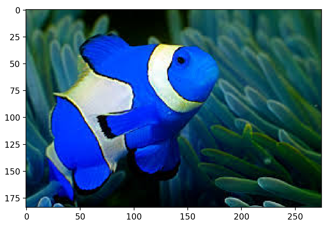
Hey, Nemo…or Dory? You’ll notice that it looks like the blue and red channels have been mixed up. In fact, OpenCV by default reads images in BGR format. You can use the cvtColor(image, flag) and the flag we looked at above to fix this:
>>> nemo = cv2.cvtColor(nemo, cv2.COLOR_BGR2RGB)
>>> plt.imshow(nemo)
>>> plt.show()
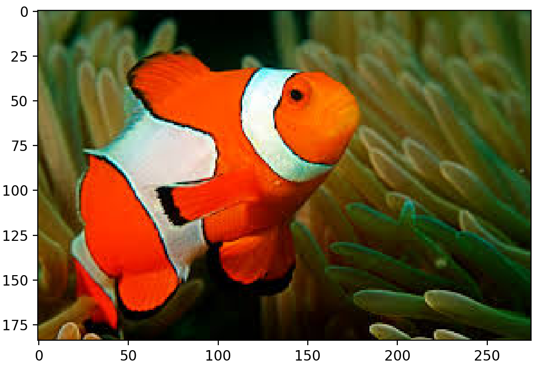
Now Nemo looks much more like himself.
Visualizing Nemo in RGB Color Space
HSV is a good choice of color space for segmenting by color, but to see why, let’s compare the image in both RGB and HSV color spaces by visualizing the color distribution of its pixels. A 3D plot shows this quite nicely, with each axis representing one of the channels in the color space. If you want to know how to make a 3D plot, view the collapsed section:
To make the plot, you will need a few more Matplotlib libraries:
>>> from mpl_toolkits.mplot3d import Axes3D
>>> from matplotlib import cm
>>> from matplotlib import colors
Those libraries provide the functionalities you need for the plot. You want to place each pixel in its location based on its components and color it by its color. OpenCV split() is very handy here; it splits an image into its component channels. These few lines of code split the image and set up the 3D plot:
>>> r, g, b = cv2.split(nemo)
>>> fig = plt.figure()
>>> axis = fig.add_subplot(1, 1, 1, projection="3d")
Now that you have set up the plot, you need to set up the pixel colors. In order to color each pixel according to its true color, there’s a bit of reshaping and normalization required. It looks messy, but essentially you need the colors corresponding to every pixel in the image to be flattened into a list and normalized, so that they can be passed to the facecolors parameter of Matplotlib scatter().
Normalizing just means condensing the range of colors from 0-255 to 0-1 as required for the facecolors parameter. Lastly, facecolors wants a list, not an NumPy array:
>>> pixel_colors = nemo.reshape((np.shape(nemo)[0]*np.shape(nemo)[1], 3))
>>> norm = colors.Normalize(vmin=-1.,vmax=1.)
>>> norm.autoscale(pixel_colors)
>>> pixel_colors = norm(pixel_colors).tolist()
Now we have all the components ready for plotting: the pixel positions for each axis and their corresponding colors, in the format facecolors expects. You can build the scatter plot and view it:
>>> axis.scatter(r.flatten(), g.flatten(), b.flatten(), facecolors=pixel_colors, marker=".")
>>> axis.set_xlabel("Red")
>>> axis.set_ylabel("Green")
>>> axis.set_zlabel("Blue")
>>> plt.show()
Here is the colored scatter plot for the Nemo image in RGB:
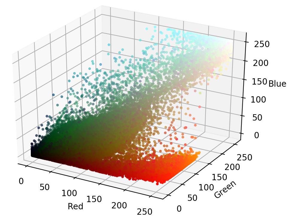
From this plot, you can see that the orange parts of the image span across almost the entire range of red, green, and blue values. Since parts of Nemo stretch over the whole plot, segmenting Nemo out in RGB space based on ranges of RGB values would not be easy.
Visualizing Nemo in HSV Color Space
We saw Nemo in RGB space, so now let’s view him in HSV space and compare.
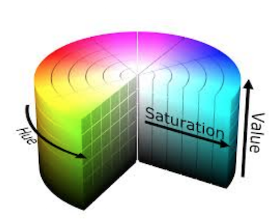
As mentioned briefly above, HSV stands for Hue, Saturation, and Value (or brightness), and is a cylindrical color space. The colors, or hues, are modeled as an angular dimension rotating around a central, vertical axis, which represents the value channel. Values go from dark (0 at the bottom) to light at the top. The third axis, saturation, defines the shades of hue from least saturated, at the vertical axis, to most saturated furthest away from the center:
To convert an image from RGB to HSV, you can use cvtColor():
>>> hsv_nemo = cv2.cvtColor(nemo, cv2.COLOR_RGB2HSV)
Now hsv_nemo stores the representation of Nemo in HSV. Using the same technique as above, we can look at a plot of the image in HSV, generated by the collapsed section below:
The code to show the image in HSV is the same as for RGB. Note that you use the same pixel_colors variable for coloring the pixels, since Matplotlib expects the values to be in RGB:
>>> h, s, v = cv2.split(hsv_nemo)
>>> fig = plt.figure()
>>> axis = fig.add_subplot(1, 1, 1, projection="3d")

>>> axis.scatter(h.flatten(), s.flatten(), v.flatten(), facecolors=pixel_colors, marker=".")
>>> axis.set_xlabel("Hue")
>>> axis.set_ylabel("Saturation")
>>> axis.set_zlabel("Value")
>>> plt.show()
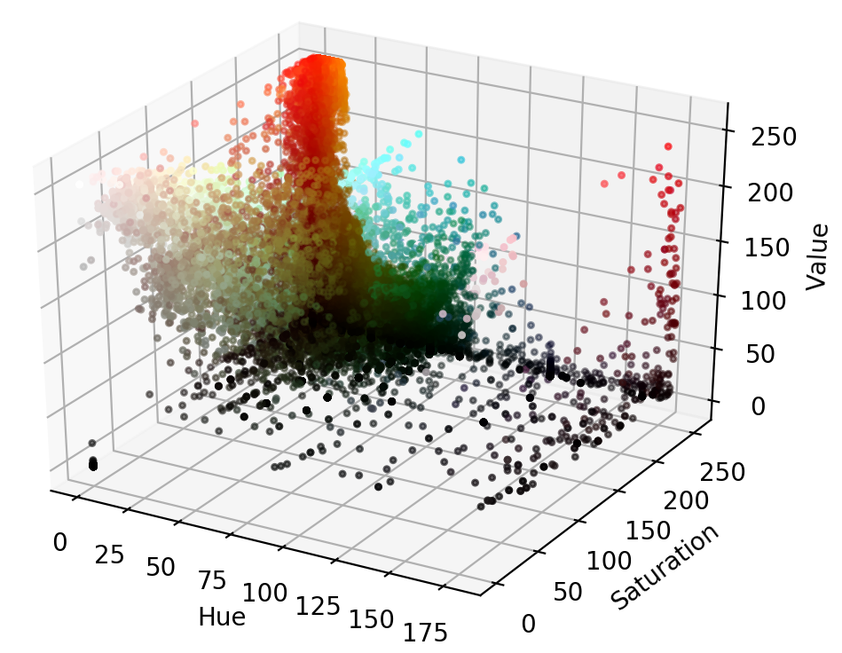
In HSV space, Nemo’s oranges are much more localized and visually separable. The saturation and value of the oranges do vary, but they are mostly located within a small range along the hue axis. This is the key point that can be leveraged for segmentation.
Picking Out a Range
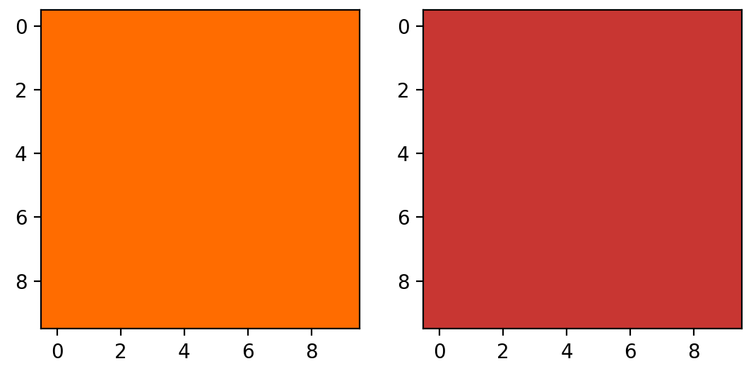
Let’s threshold Nemo just based on a simple range of oranges. You can choose the range by eyeballing the plot above or using a color picking app online such as this RGB to HSV tool. The swatches chosen here are a light orange and a darker orange that is almost red:
>>> light_orange = (1, 190, 200)
>>> dark_orange = (18, 255, 255)
If you want to use Python to display the colors you chose, click on the collapsed section:
A simple way to display the colors in Python is to make small square images of the desired color and plot them in Matplotlib. Matplotlib only interprets colors in RGB, but handy conversion functions are provided for the major color spaces so that we can plot images in other color spaces:
>>> from matplotlib.colors import hsv_to_rgb
Then, build the small 10x10x3 squares, filled with the respective color. You can use NumPy to easily fill the squares with the color:
>>> lo_square = np.full((10, 10, 3), light_orange, dtype=np.uint8) / 255.0
>>> do_square = np.full((10, 10, 3), dark_orange, dtype=np.uint8) / 255.0
Finally, you can plot them together by converting them to RGB for viewing:
>>> plt.subplot(1, 2, 1)
>>> plt.imshow(hsv_to_rgb(do_square))
>>> plt.subplot(1, 2, 2)
>>> plt.imshow(hsv_to_rgb(lo_square))
>>> plt.show()
That produces these images, filled with the chosen colors:
Once you get a decent color range, you can use cv2.inRange() to try to threshold Nemo. inRange() takes three parameters: the image, the lower range, and the higher range. It returns a binary mask (an ndarray of 1s and 0s) the size of the image where values of 1 indicate values within the range, and zero values indicate values outside:
>>> mask = cv2.inRange(hsv_nemo, light_orange, dark_orange)
To impose the mask on top of the original image, you can use cv2.bitwise_and(), which keeps every pixel in the given image if the corresponding value in the mask is 1:
>>> result = cv2.bitwise_and(nemo, nemo, mask=mask)
To see what that did exactly, let’s view both the mask and the original image with the mask on top:
>>> plt.subplot(1, 2, 1)
>>> plt.imshow(mask, cmap="gray")
>>> plt.subplot(1, 2, 2)
>>> plt.imshow(result)
>>> plt.show()
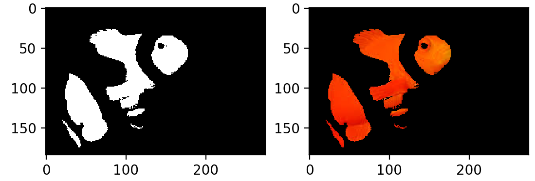
There you have it! This has already done a decent job of capturing the orange parts of the fish. The only problem is that Nemo also has white stripes… Fortunately, adding a second mask that looks for whites is very similar to what you did already with the oranges:
>>> light_white = (0, 0, 200)
>>> dark_white = (145, 60, 255)
Once you’ve specified a color range, you can look at the colors you’ve chosen:
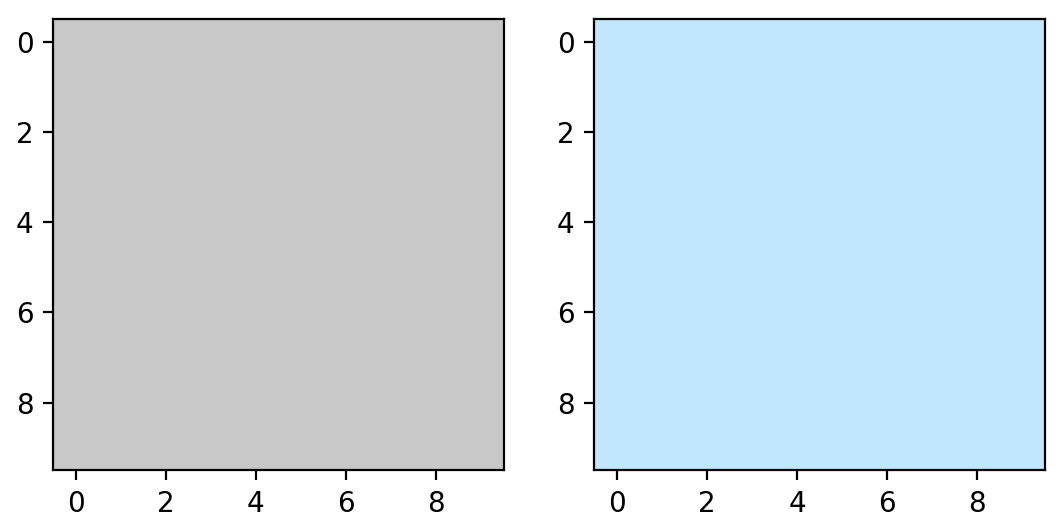
To display the whites, you can take the same approach as we did previously with the oranges:
>>> lw_square = np.full((10, 10, 3), light_white, dtype=np.uint8) / 255.0
>>> dw_square = np.full((10, 10, 3), dark_white, dtype=np.uint8) / 255.0

>>> plt.subplot(1, 2, 1)
>>> plt.imshow(hsv_to_rgb(lw_square))
>>> plt.subplot(1, 2, 2)
>>> plt.imshow(hsv_to_rgb(dw_square))
>>> plt.show()
The upper range I’ve chosen here is a very blue white, because the white does have tinges of blue in the shadows. Let’s create a second mask and see if it captures Nemo’s stripes. You can build a second mask the same way as you did the first:
>>> mask_white = cv2.inRange(hsv_nemo, light_white, dark_white)
>>> result_white = cv2.bitwise_and(nemo, nemo, mask=mask_white)

>>> plt.subplot(1, 2, 1)
>>> plt.imshow(mask_white, cmap="gray")
>>> plt.subplot(1, 2, 2)
>>> plt.imshow(result_white)
>>> plt.show()
Not bad! Now you can combine the masks. Adding the two masks together results in 1 values wherever there is orange or white, which is exactly what is needed. Let’s add the masks together and plot the results:
>>> final_mask = mask + mask_white

>>> final_result = cv2.bitwise_and(nemo, nemo, mask=final_mask)
>>> plt.subplot(1, 2, 1)
>>> plt.imshow(final_mask, cmap="gray")
>>> plt.subplot(1, 2, 2)
>>> plt.imshow(final_result)
>>> plt.show()
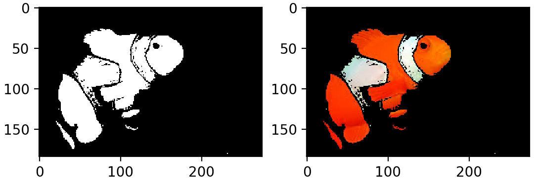
Essentially, you have a rough segmentation of Nemo in HSV color space. You’ll notice there are a few stray pixels along the segmentation border, and if you like, you can use a Gaussian blur to tidy up the small false detections.
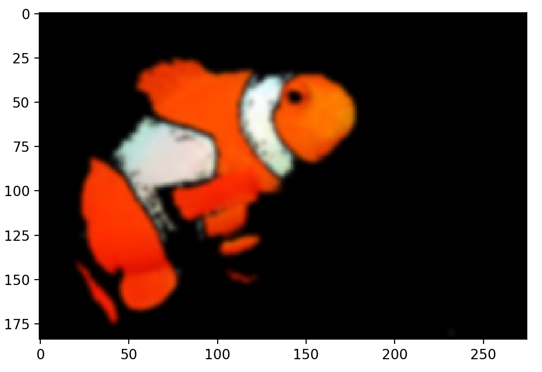
A Gaussian blur is an image filter that uses a kind of function called a Gaussian to transform each pixel in the image. It has the result of smoothing out image noise and reducing detail. Here’s what applying the blur looks like for our image:
>>> blur = cv2.GaussianBlur(final_result, (7, 7), 0)
>>> plt.imshow(blur)
>>> plt.show()
Does This Segmentation Generalize to Nemo’s Relatives?
Just for fun, let’s see how well this segmentation technique generalizes to other clownfish images. In the repository, there’s a selection of six images of clownfish from Google, licensed for public use. The images are in a subdirectory and indexed nemoi.jpg, where i is the index from 0-5.
First, load all Nemo’s relatives into a list:
path = "./images/nemo"

nemos_friends = []
for i in range(6):
   friend = cv2.cvtColor(cv2.imread(path + str(i) + ".jpg"), cv2.COLOR_BGR2RGB)
   nemos_friends.append(friend)
You can combine all the code used above to segment a single fish into a function that will take an image as input and return the segmented image. Expand this section to see what that looks like:
Here is the segment_fish() function:
def segment_fish(image):
    ''' Attempts to segment the clownfish out of the provided image '''

    # Convert the image into HSV
    hsv_image = cv2.cvtColor(image, cv2.COLOR_RGB2HSV)

    # Set the orange range
    light_orange = (1, 190, 200)
    dark_orange = (18, 255, 255)

    # Apply the orange mask
    mask = cv2.inRange(hsv_image, light_orange, dark_orange)

    # Set a white range
    light_white = (0, 0, 200)
    dark_white = (145, 60, 255)

    # Apply the white mask
    mask_white = cv2.inRange(hsv_image, light_white, dark_white)

    # Combine the two masks
    final_mask = mask + mask_white
    result = cv2.bitwise_and(image, image, mask=final_mask)

    # Clean up the segmentation using a blur
    blur = cv2.GaussianBlur(result, (7, 7), 0)
    return blur
With that useful function, you can then segment all the fish:
results = [segment_fish(friend) for friend in nemos_friends]
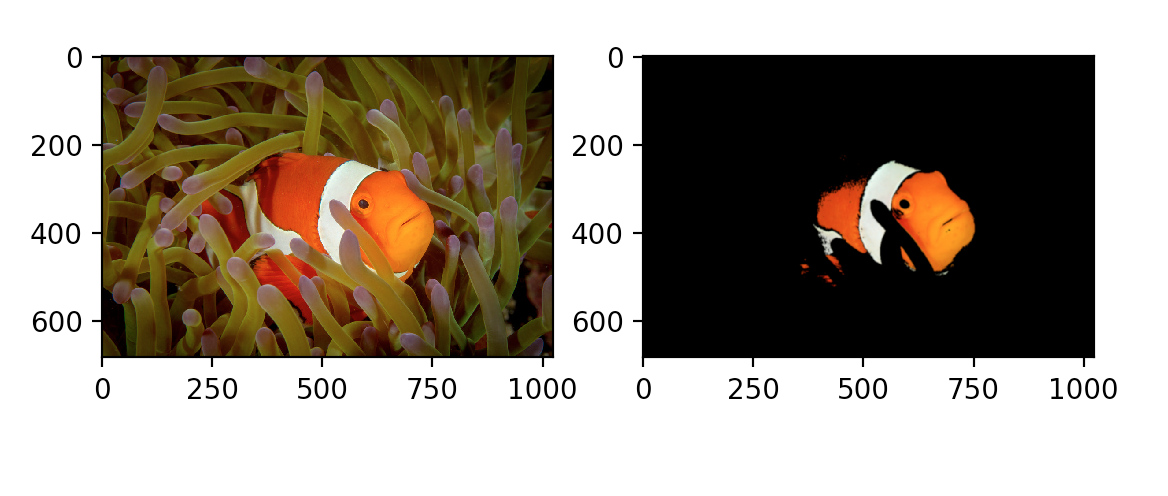
Let’s view all the results by plotting them in a loop:
for i in range(1, 6):
    plt.subplot(1, 2, 1)
    plt.imshow(nemos_friends[i])
    plt.subplot(1, 2, 2)
    plt.imshow(results[i])
    plt.show()
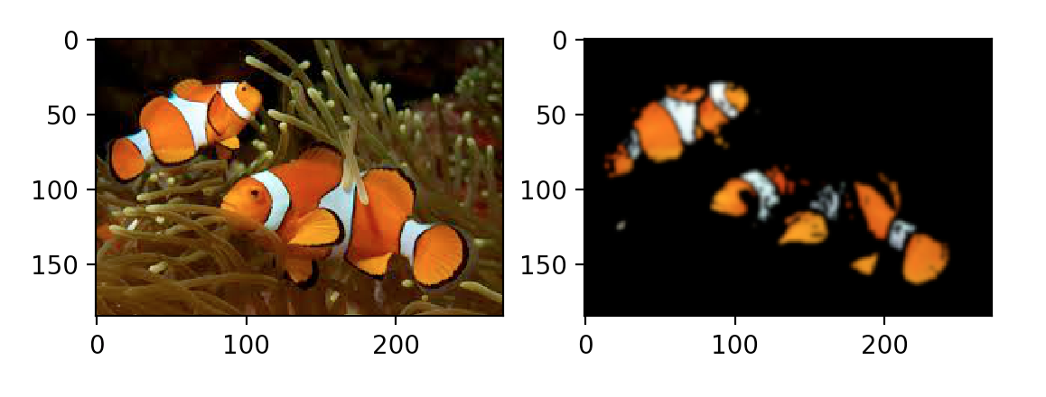
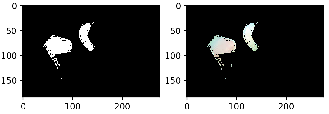
The foreground clownfish has orange shades darker than our range.
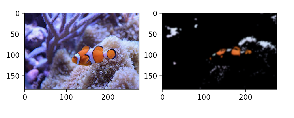
The shadowed bottom half of Nemo’s nephew is completely excluded, but bits of the purple anemone in the background look awfully like Nemo’s blue tinged stripes…
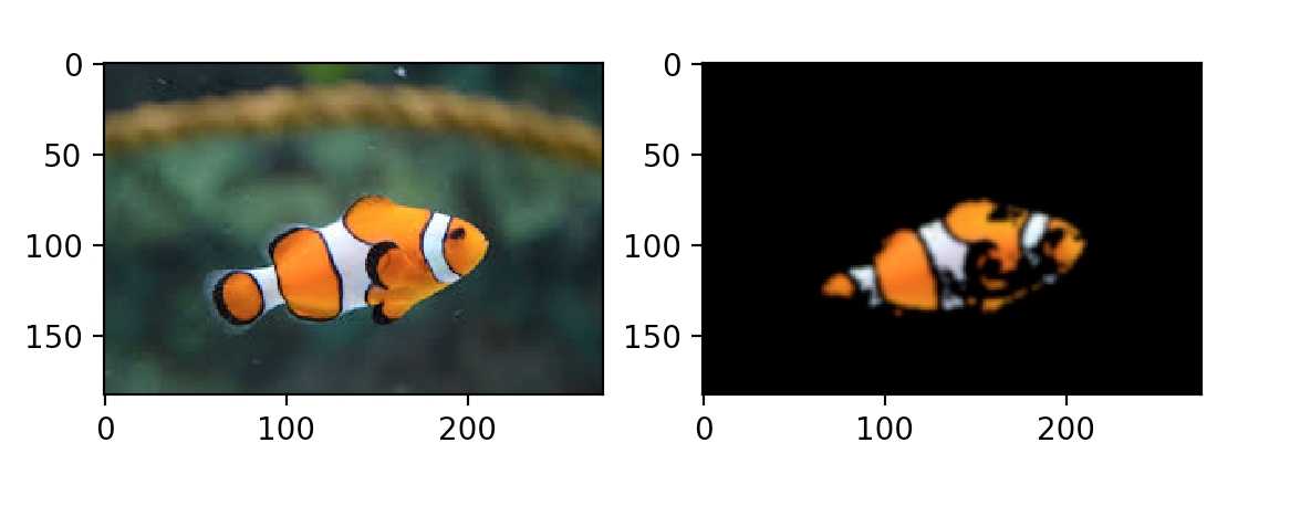
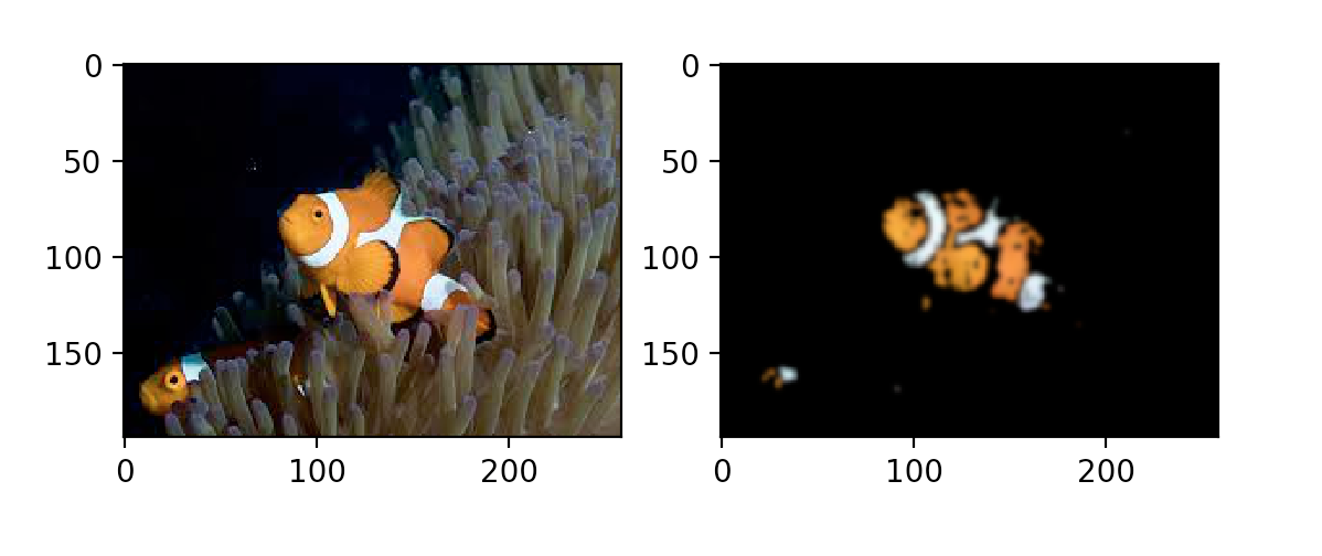
Overall, this simple segmentation method has successfully located the majority of Nemo’s relatives. It is clear, however, that segmenting one clownfish with particular lighting and background may not necessarily generalize well to segmenting all clownfish.
Conclusion
In this tutorial, you’ve seen what a few different color spaces are, how an image is distributed across RGB and HSV color spaces, and how to use OpenCV to convert between color spaces and segment out ranges.
Altogether, you’ve learned how a basic understanding of how color spaces in OpenCV can be used to perform object segmentation in images, and hopefully seen its potential for doing other tasks as well. Where lighting and background are controlled, such as in an experimental setting or with a more homogeneous dataset, this segmentation technique is simple, fast, and reliable.